DBScan

DBScan is a useful density-based clustering algorithm for unsupervised learning. Unlike KMeans Clustering, DBScan can identify irregularly shaped clusters and is also resilient to noise. I go over the algorithm, its implementation, and two simple experiments. See the interactive Colab Notebook for more.

Overview

DBScan stands for Density Based Spatial Clustering of Applications with Noise. The core idea of DBScan is that it classifies clusters as groups of points that are “connected” through their “neighbors”. All points that are reachable from a specific point through its neighbors following a certain rule are classified as a single cluster. We find all possible clusters like this and label the remaining points as noise. The algorithm takes two parameters: epsilon and minimum_neighbors.

Terminology

To make these ideas more concrete, we must define some simple terms. We must understand what it means for points to be “neighbors”; three ways of classifying points: “core points”, “border points”, and “noise points”; and finally what it means for points to be “connected”.

Neighbors: All points within epsilon of a point p are considered neighbors of p. Different notions of distance may be used, but generally we use Euclidean distance, which is the norm of the difference between two points.

A point is classified in one of the following three categories depending on the number of neighbors that it has.

Core Points: A point is a core point if it has at least minimum_neighbors neighbors.
Border Points: A point is a border point if it has at least one neighbor but less than minimum_neighbors neighbors.
Noise Points: A point is a noise point if it has no neighbors.

There are two main notions of points being connected.

Directly Reachable: A point q is directly reachable from a point p if p is a core point and q is a neighbor of p. We only say that points are directly reachable from core points.
Reachable: A point q is reachable from a point p if p is a core point and there is a path from p to q where each point on the path is directly reachable from the previous point. This means that we can reach q from p through p’s neighbors, but only if those neighbors are core points. Point q is not reachable from p if we must go through neighbors that are border points.

The Algorithm

With these terms in place, we can now better understand the algorithm. A single cluster consists of all points that are “reachable” from a “core point” p. We can find all points reachable from p through a searching algorithm, which I describe in the next paragraph. By doing this searching process from p, we have exhaustively found the entire cluster. We repeat this on all unlabeled core points until all clusters are found. The remaining points are classified as noise and the algorithm returns the labels for every data point. Note that border points may finally be classified as noise if they are not reachable from any core point.

I like to think of the process of identifying a cluster as expanding a search tree from p. Point p is the root node of the tree. All of its children are its neighbors. We then further expand the tree by adding the children of any core point nodes until it can no longer be expanded. This complete tree will consist of all points reachable from p and is therefore a single cluster. If we used any core point in the tree as the root node we would obtain the same cluster.

The process of identifying all points in a cluster can then be thought of as running a search algorithm from p such as Breadth First Search or Depth First Search. I will use BFS in my implementation by storing all neighboring points in a queue and searching them in FIFO (First In First Out) order.

This yields the following algorithm:

1. Pick a point p that has not yet been labeled and identify its neighboring points with respect to epsilon. If it is a core point, assign it to a new cluster, c, and continue. If it is noise or a border point, assign it to the noise cluster and repeat step 1 on a new point.
2. Add all neighboring points of the core point p to a queue and assign them to cluster c.
3. Remove a point from the queue and assign it to cluster c if it has not been assigned to a non-noise cluster yet. If it is a core point, add all of its neighboring points to the queue. Repeat this step until the queue is empty.
4. Repeat steps 1-3 until all points have been assigned to a cluster or as noise.

The Code

I implemented this algorithm with Python and numpy. I break this code up into three functions: neighbor_points finds all the neighbors of a point; cluster labels all points in a single cluster given a core point; DBScan is the final algorithm that clusters all the data. See the interactive Colab notebook to see these algorithms implemented and to play around with them yourself.

Data is an n by d numpy array where n is the number of data points and d is the number of features for each point.

The below code returns all points that neighbor a given point. Throughout my code, I work with the indices of points rather than the points themselves. I calculate the distance between every point and p simultaneously using broadcasting. This leads to a significant speedup compared to a naive implementation using a for loop. In particular, my first experiment with DBScan took an average of 327 milliseconds with this implementation, as opposed to 8.21 seconds with a naive implementation.

def neighbor_points(data, point_idx, eps):
  '''
  Given a data matrix and point_idx, returns the indices of all points
  within eps Euclidean distance of the point corresponding to point_idx.
  '''
  distances = np.linalg.norm(data - data[point_idx], axis=1)
  return np.where(distances <= eps)[0].tolist()

The below code updates cluster_labels to include all points in a new cluster, c, found by expanding from a core point. Cluster_labels may already have labels in it from the dbscan function.

The list neighboring_points is used as a queue. We check each point in it following the FIFO principle. If a point is considered noise, which we indicate by -1, we assign it to cluster c. In this case, we know the point is a border point. If the point hasn’t been assigned a cluster yet, which we indicate by 0, we assign it to cluster c. If it is a core point, we add its neighbors to the queue. This process is repeated until the queue is exhausted.

def cluster(data, neighboring_points, cluster_labels, point_idx, c, eps, m):
  '''
  Grows a cluster with label c from point.
  Updates cluster_labels to include all points in cluster c
  '''
  cluster_labels[point_idx] = c
  i = 0
  while i < len(neighboring_points):
    np_idx = neighboring_points[i]
    if cluster_labels[np_idx] == -1:
      cluster_labels[np_idx] = c
    elif cluster_labels[np_idx] == 0:
      cluster_labels[np_idx] = c
      npts2 = neighbor_points(data, np_idx, eps)
      if len(npts2) >= m:
        neighboring_points = neighboring_points + npts2
    i += 1

The below code is the final DBScan algorithm.

We first initialize cluster_labels as an array of zeroes where each entry corresponds to a data point. Zero is used as a special label to tell us that a point has not been labeled yet. When cluster_labels is returned, no point will be labeled with a zero.

We iterate through every point in the data, skipping over points that have already been labeled. If a point has not been labeled yet, we find all of its neighboring points. If it is a core point, we form one cluster by using cluster to label all points reachable from it. Otherwise, we assign the point to cluster -1, which we use to mark noise. Border points assigned to cluster -1 may be assigned to a new cluster later if they are reachable from a core point.

def dbscan(data, eps, m, verbose = False):
    '''
  Given data, eps (used to determine neighbors), m (minimum points to be a core point).
  Returns an array where every entry is a label corresponding to an entry of data.
  If the label is -1, the point is considered noise. Otherwise it is in a cluster.
  '''
  cluster_labels = np.zeros(data.shape[0])
  c = 1
  for i in range(data.shape[0]):
    if cluster_labels[i] == 0: # only do this if the point has not been assigned a cluster yet
      npts = neighbor_points(data, i, eps) # this returns indices of neighboring points
      if len(npts) < m: # if the point is a border or noise point
        cluster_labels[i] = -1 # -1 is the noise cluster here
        # Points with no neighbors will remain in this cluster, while border points may change clusters
      if len(npts) >= m: # if the point is a core point
        cluster(data, npts, cluster_labels, i, c, eps, m)
        if verbose:
          print(cluster_labels)
          print("Clustering Done")
        c += 1
  return cluster_labels
  

Experiments: Simple Clustered Data

Let’s test DBScan on the following 2-dimensional data. For more details on this experiment, or to play around with it yourself, see the Colab Notebook.

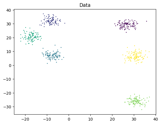
I used DBScan with eps = 4 and m = 3. It’s important to realize that DBScan is sensitive to hyperparameters. It requires experimentation and possible domain knowledge to choose them well. I got the following result, which sure enough, matches our expectations. The only difference is a singular point labeled as noise, which makes sense upon inspection.

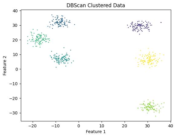
I ran KMeans on the same data and also got the same result (without the singular noise point). However, for KMeans, I had to specify the number of clusters in advance.

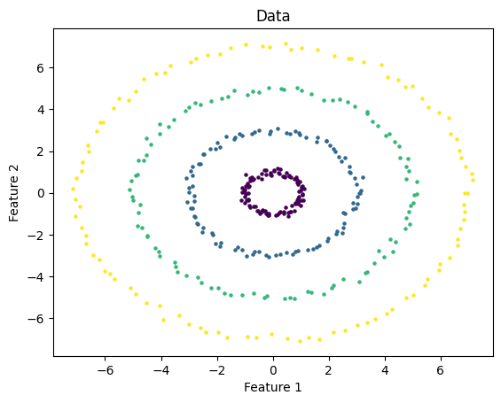
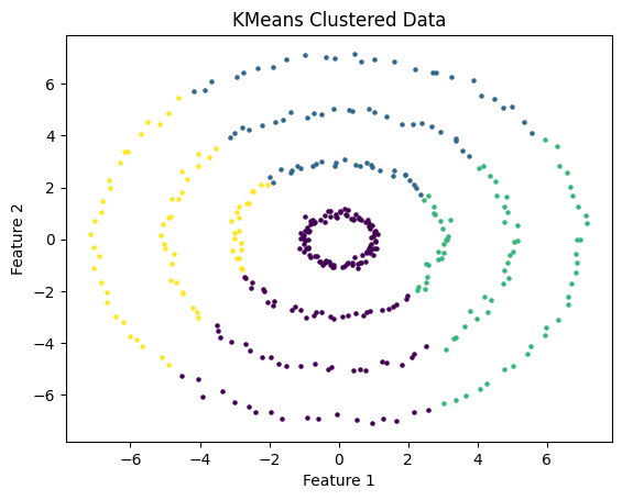
Experiments: Ring Data

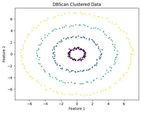
Where DBScan really shines is in its ability to recognize clusters that have irregular shapes. I test DBScan on the following data which consists of a series of concentric rings.

I used DBScan with eps = 1 and m = 3. As you can see, the algorithm successfully identified the clusters.

On the other hand, KMeans completely failed to recognize the clusters in this data. This is because KMeans is only able to work on clusters that are roughly spherically symmetric around a centroid. In this data, the clusters can not be defined as such.

Future Experiments

The experiments that I conducted were fairly simple, but DBScan is powerful enough to work on much more interesting data. I suggest as an exercise evaluating the following questions.

• How does DBScan perform when there is significant noise? You can try implementing the experiments that I did but with more noise added. In the Colab Notebook, I implemented a basic noise generation function that you can play with. A possible issue is that with eps too large, points that seem like noise may be clustered together, resulting in numerous clusters of noise.

• How does DBScan perform on higher dimensional data? The experiments that I did work in 2-dimensions, but DBScan can be used on much higher dimensions, without much difference in time efficiency. You can visualize these experiments by using a dimensionality reduction technique such as PCA or t-SNE to project the data down into 2 or 3 dimensions.